Chapter 10 Parametric statistics
10.1 Introduction
The majority of statistical tools that we use in this book share one important feature: they are underpinned by a mathematical model of some kind. Because a mathematical model is lurking in the background, this particular flavour of statistics is known as parametric statistics. In this context, the word ‘parametric’ refers to the fact that the behaviour of such a model is defined by one or more quantities known as ‘parameters’.
We aren’t going to study the mathematical details of these models in any detail. This isn’t a maths book. However, it’s important to at least understand the assumptions underlying a statistical model. Mathematical assumptions are the aspects of a system that we accept as true, or at least nearly true. If these aren’t reasonable for a given situation, we can’t be sure that the results of the corresponding analysis (e.g. a statistical test) will be reliable. We always need to evaluate the assumptions of an analysis to determine whether or not we trust it.
Ultimately, we want to understand, in rough terms at least, how a model and its assumptions lead to a particular statistical test. We explored a number of concepts from frequentist statistics in the last few chapters, such as sampling variation, null distributions, and p-values. These ideas will crop up time and time again throughout the book. By thinking about models and their assumptions we can begin to connect the abstract ideas in the last few chapters to the practical aspects of ‘doing statistics’.
10.2 Mathematical models
A mathematical model is a description of a system using the language and concepts of mathematics. A statistical model is a particular class of mathematical model that describes how samples of data are generated from a hypothetical population. We’re going to consider only a small subset of the huge array of statistical models people routinely use.
In conceptual terms, the statistical models we use describe data in terms of a systematic component and a random component:
\[\text{Observed Data} = \text{Systematic Component} + \text{Random Component}\]
The systematic component of a model describes the structure, or the relationships, in the data. When people refer to ‘the model’, this is the bit they usually care about. The random component captures the left over “noise” in the data. This is essentially the part of the data that the systematic component of the model fails to describe.
This is best understood by example. In what follows we’re going to label the individual values in the sample \(y_i\). The \(i\) in this label indexes the individual values; it takes values 1, 2, 3, 4, … and so on. We can think of the collection of the \(y_i\)’s as the variable we’re interested in.
The simplest kind of model we might consider is one that describes a single variable. A model for these data can be written: \(y_i = a + \epsilon_i\). With this model, the systematic part is given by \(a\). This is usually the population mean. The random component is given by \(\epsilon_i\). The \(\epsilon_i\) is a model variable that describes how the individual values deviate from the mean.
A more complicated model is one that considers the relationship between the values of \(y_i\) and another variable. We’ll call this second variable \(x_i\). A model for these data could be written as: \(y_i = a + b \times x_i + \epsilon_i\). The \(a + b \times x_i\) bit of this—the equation of a straight line with an intercept \(a\) and slope \(b\)—is the systematic component. The random component is given by the \(\epsilon_i\). Here, this model variable describes how the individual values deviate from the line.
Each of these two descriptions represents a partially specified statistical model. We need to make one more assumption to complete them. What is missing is a description of the distribution of the \(\epsilon_i\). In rough terms, a statement about a variable’s distribution is a statement how likely different values are. In this book, this assumption is almost always the same: we assume that the \(\epsilon_i\) are drawn from a normal distribution…
10.3 The normal distribution
Most people will come across the normal distribution at one point or another, though they may not realise it at the time. Here’s a histogram of 100000 values drawn from a normal distribution (the details don’t matter here):
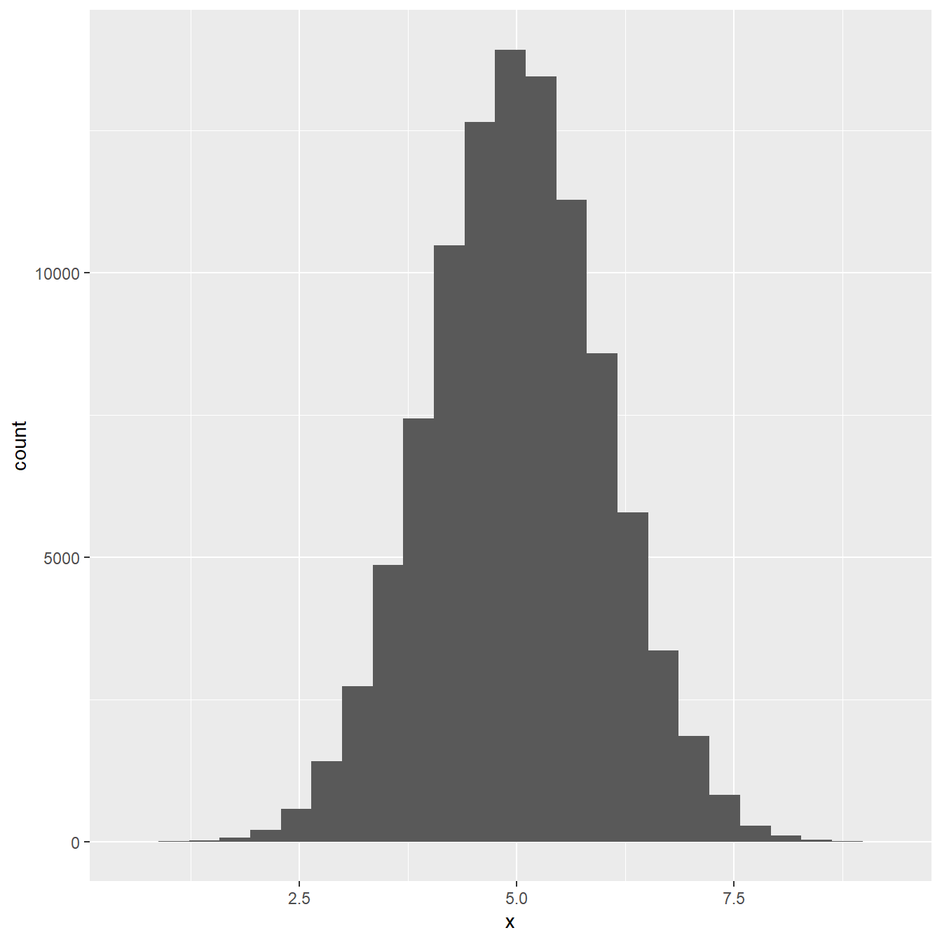
Figure 10.1: Distribution of a large sample of normally distributed variable
Does that look familiar? The normal distribution is sometimes called the ‘Gaussian distribution’, or more colloquially, the ‘bell-shaped curve’. We don’t have time in this book to really study this distribution in much detail, nor is it really necessary that we do this. We’ll just list some key facts about the normal distribution that we need to refer to from time to time:
The normal distribution is appropriate for numeric variables measured on an interval or ratio scale. Strictly speaking, the variable should also be continuous, though a normal distribution can provide a decent approximation for some kinds of discrete numeric data.
The normal distribution is completely described by its mean (a measure of ‘central tendency’) and its standard deviation (a measure of ‘dispersion’). If we know these two quantities for a particular normal distribution, we know everything there is to know about that distribution.
If a variable is normally distributed, then about 95% of its values will fall inside an interval that is 4 standard deviations wide: the upper bound is equal to the \(\text{Mean} + 2 \times \text{S.D.}\); the lower bound is equal to \(\text{Mean} - 2 \times \text{S.D.}\).
When we add or subtract two normally distributed variables to create a new variable, the resulting variable will also be normally distributed. Similarly, if we multiply a normally distributed by a number to create a new variable, the resulting variable will still be normally distributed.
The mathematical properties of the normal distribution are very well understood and many of these properties make the distribution easy to work with. This has made it possible for mathematicians to work out how the sampling distribution of means and variances behave when the underlying variables are normally distributed. This knowledge underpins many of the statistical tests we use in this book.
10.3.1 Standard error of the mean
Let’s consider a simple example. Say that we want to estimate the standard error of the sampling distribution of a mean. If we’re happy to assume that the sample was drawn from a normal distribution, then there’s no need to resort to computationally expensive techniques like bootstrapping to work this out. Instead, there is a well-known formula for calculating the standard error we need. If \(s^2\) is the variance of the sample, and \(n\) is the sample size, the standard error is given by:
\[\text{Standard error of the mean} = \sqrt{\frac{s^2}{n}}\]
That’s it, if we know the variance and the size of a sample, it’s easy to estimate the standard error of its mean. In fact, as a result of rule #4 above, we can calculate the standard error of any quantity that involves adding or subtracting the means of samples drawn from normal distributions.
10.3.2 The t distribution
The normal distribution is usually the first distribution people learn about. The reasons for this are: 1) it crops up a lot because of something called ‘the central limit theorem’ and 2) many other distributions are related to the normal distribution. One of the most important of these ‘other distributions’ is Student’s t-distribution1. This arises when…
we take a sample from a normally distributed variable,
estimate the population mean from the sample,
and then divide the mean by its standard error (i.e. calculate: mean / s.e.).
The sampling distribution of this new quantity has a particular form. It follows a Student’s t-distribution. Student’s t-distribution arises all the time in relation to means. For example, what happens if we take samples from a pair of normal distributions, calculate the difference between their estimated means, and then divide this difference by its standard error? The sampling distribution of the scaled difference between means also follows a Student’s t-distribution.
Because it involves rescaling a mean by its standard error, the form of the resulting t-distribution only depends on one thing: the sample size. This may not sound like an important result, but it is because it allows us to construct simple statistical tests to evaluate differences between means. We’ll use this result in the next two chapters as we learn about so-called ‘t-tests’.
Why is it called Student’s t? The t-distribution was discovered by W.G. Gosset, a statistician employed by the Guinness Brewery. He published his statistical work under the pseudonym of ‘Student’, because Guinness would have claimed ownership of his work if he had used his real name.↩︎