-
Bookdown thesis examples (15 Feb 2022)
Booking calenders and web intergration (13 Feb 2022)
Jekyll metadata (08 Feb 2022)
Adding links in Jekyll websites (25 Nov 2021)
A good way to manage and document a large number of resources. This is done in beautiful jekyll using liqud tags. TO include a full list of all my blog posts so far.
<article>
<h2>
<a href="/2022-03-10-Resolution-and-pixels/">
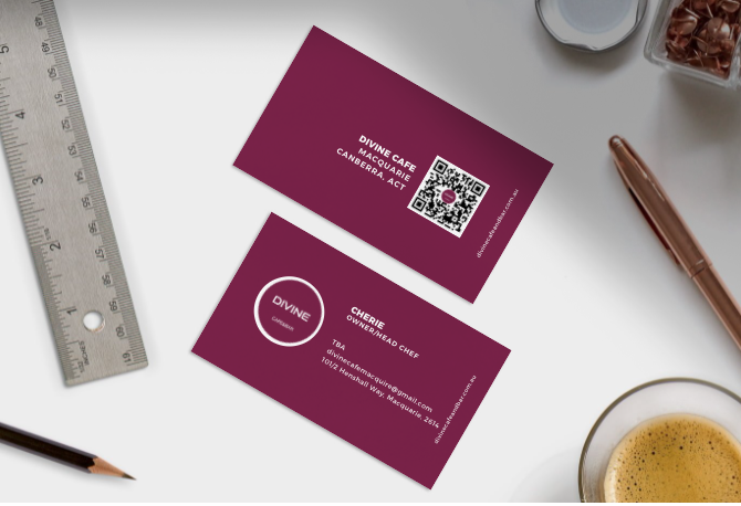
Creating business cards
</a>
</h2>
<time datetime="2022-03-10">10 March 2022</time>
[Resolution vs. Image Size Explained (GIMP Tutorial)](https://youtu.be/4rhVKBp4Fe4)
https://youtu.be/4rhVKBp4Fe4
## General steps
There are many different online tools that can be used to create design objects such as in [https://desygner.com/](https://desygner.com/) and [Canvas](https://www.canva.com/)
## Other blog posts
[coming]
<div class="post"><ul>
{% for post in site.tags["business"] %}
<a href="{{ post.url }}">{{ post.title }}</a> ({{ post.date | date_to_string }})<br>
{{ post.description }}
{% endfor %}
</ul></div>
</article>
<article>
<h2>
<a href="/2022-02-23-business-card-development/">
Creating business cards
</a>
</h2>
<time datetime="2022-02-23">23 February 2022</time>

## General steps
There are many different online tools that can be used to create design objects such as in [https://desygner.com/](https://desygner.com/) and [Canvas](https://www.canva.com/)
## Other blog posts
[coming]
<div class="post"><ul>
{% for post in site.tags["business"] %}
<a href="{{ post.url }}">{{ post.title }}</a> ({{ post.date | date_to_string }})<br>
{{ post.description }}
{% endfor %}
</ul></div>
</article>
<article>
<h2>
<a href="/2022-02-19-building-a-qr-code/">
Building a QR code
</a>
</h2>
<time datetime="2022-02-19">19 February 2022</time>
[QR codes](https://en.wikipedia.org/wiki/QR_code) have been all the rage in the past few years. Below are my simple steps to quickly making a single QR code either online, using a design application (e.g. Canvas) or through R.

## General steps
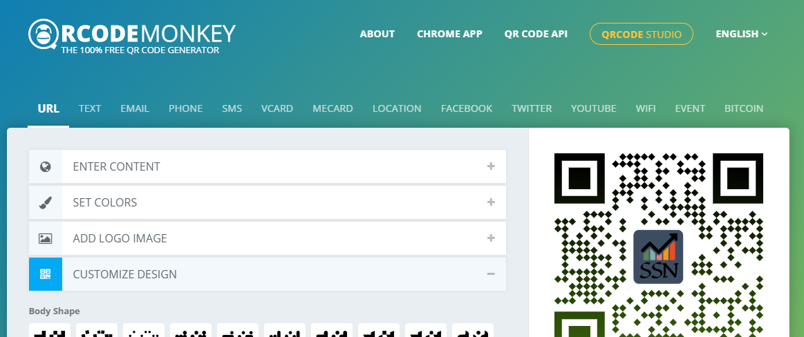
A straightforward way to generate a QR code is to pick one of the many online tools to do it. Here are a few I have used (note some of the links might be broken):
- One option [here](https://www.qr-code-generator.com/)
- Another one [here](https://www.the-qrcode-generator.com/): This one is a little simpler
- I used this [one](https://www.qrcode-monkey.com/): I liked this one because of easy custom image insert but im sure they are all “much of a muchness”
- Medium blog https://medium.com/@gliechtenstein/build-a-qrcode-barcode-scanning-app-with-26-lines-of-json-b83453d39197
- https://www.qrcode-monkey.com/#about
##### Outcome
...try scanning it??

## Tutorials
There could be a bit to come here....
### Further points
- There are different things that QR codes can be used for including url links, pdfs,
- Here is an online [https://www.qrstuff.com/ scanner](https://www.qrstuff.com/scan)
### An extention
I have used a simple design app made for data scientists and social media advertisers to make simple and quick designs. It is called [desygner](https://desygner.com). This is not the only option and paint will do but this free (basics anyway) gets the image sizes closer than I know how with my mind and a "paint" brush.
##### And Another
This same tech is used for creating and catalogueing databases (even jekyll ones).
- [barcodelib](https://github.com/barnhill/barcodelib/)
- [zint](https://github.com/zint/zint)
- [QR-generator](https://github.com/nayuki/QR-Code-generator)
</article>
<article>
<h2>
<a href="/2022-02-15-bookdown-thesis-templates/">
Bookdown thesis examples
</a>
</h2>
<time datetime="2022-02-15">15 February 2022</time>
# Overview
Using RMarkdown and RStudio to render static documents (pdf, html, docx) can be helpful for incorperating style rules and reproducible methods. It can be just as painful if complex extensions and modifications fail to work as the complexity of the pipeline can make problem solving challenging. Below are a collection of packages that work around writing thesis documents using multiple RMarkdown files in R. I have also created a template for UC thesis documents (`ucdown`) that can be found on github under `davan690/ucdown`. To install ucdown run the following command in RStudio:
[coming...]
# Output Formats
The **bookdown** package primarily supports three types of output formats: HTML, LaTeX/PDF, and e-books. In this chapter, we introduce the possible options for these formats. Output formats can be specified either in the YAML metadata of the first Rmd file of the book, or in a separate YAML file named `_output.yml` under the root directory of the book. Here is a brief example of the former (output formats are specified in the `output` field of the YAML metadata):
```yaml
---
title: "An Impressive Book"
author: "Li Lei and Han Meimei"
output:
bookdown::gitbook:
  lib_dir: assets
  split_by: section
  config:
    toolbar:
      position: static
bookdown::pdf_book:
  keep_tex: yes
bookdown::html_book:
  css: toc.css
documentclass: book
---
Here is an example of _output.yml\index{_output.yml}:
bookdown::gitbook:
lib_dir: assets
split_by: section
config:
toolbar:
position: static
bookdown::pdf_book:
keep_tex: yes
bookdown::html_book:
css: toc.css
In this case, all formats should be at the top level, instead of under an output field. You do not need the three dashes --- in _output.yml.
The main difference between rendering a book (using bookdown) with rendering a single R Markdown document (using rmarkdown) to HTML\index{HTML} is that a book will generate multiple HTML pages by default — normally one HTML file per chapter. This makes it easier to bookmark a certain chapter or share its URL with others as you read the book, and faster to load a book into the web browser. Currently we have provided a number of different styles for HTML output: the GitBook style, the Bootstrap style, and the Tufte style.
The GitBook style was borrowed from GitBook\index{GitBook}, a project launched by Friendcode, Inc. (https://www.gitbook.com) and dedicated to helping authors write books with Markdown. It provides a beautiful style, with a layout consisting of a sidebar showing the table of contents on the left, and the main body of a book on the right. The design is responsive to the window size, e.g., the navigation buttons are displayed on the left/right of the book body when the window is wide enough, and collapsed into the bottom when the window is narrow to give readers more horizontal space to read the book body.
We have made several improvements over the original GitBook project. The most significant one is that we replaced the Markdown engine with R Markdown v2 based on Pandoc, so that there are a lot more features for you to use when writing a book:
We have also added some useful features in the user interface that we will introduce in detail soon. The output format function for the GitBook style in bookdown is gitbook(). Here are its arguments:
```{r gitbook-args, code=formatR::usage(bookdown::gitbook, output=FALSE, fail=’none’), eval=FALSE, R.options=list(width=50)}
Most arguments are passed to `rmarkdown::html_document()`, including `fig_caption`, `lib_dir`, and `...`. You can check out the help page of `rmarkdown::html_document()` for the full list of possible options. We strongly recommend you to use `fig_caption = TRUE` for two reasons: 1) it is important to explain your figures with captions; 2) enabling figure captions means figures will be placed in floating environments when the output is LaTeX, otherwise you may end up with a lot of white space on certain pages. The format of figure/table numbers depends on if sections are numbered or not: if `number_sections = TRUE`, these numbers will be of the format `X.i`, where `X` is the chapter number, and `i` in an incremental number; if sections are not numbered, all figures/tables will be numbered sequentially through the book from 1, 2, ..., N. Note that in either case, figures and tables will be numbered independently.

Among all possible arguments in `...`, you are most likely to use the `css` argument to provide one or more custom CSS files to tweak the default CSS style. There are a few arguments of `html_document()` that have been hard-coded in `gitbook()` and you cannot change them: `toc = TRUE` (there must be a table of contents), `theme = NULL` (not using any Bootstrap themes), and `template` (there exists an internal GitBook template).

Please note that if you change `self_contained = TRUE` to make self-contained HTML pages, the total size of all HTML files can be significantly increased since there are many JS and CSS files that have to be embedded in every single HTML file.

Besides these `html_document()` options, `gitbook()` has three other arguments: `split_by`, `split_bib`, and `config`. The `split_by` argument specifies how you want to split the HTML output into multiple pages, and its possible values are:

- `rmd`: use the base filenames of the input Rmd files to create the HTML filenames, e.g., generate `chapter3.html` for `chapter3.Rmd`.
- `none`: do not split the HTML file (the book will be a single HTML file).
- `chapter`: split the file by the first-level headers.
- `section`: split the file by the second-level headers.
- `chapter+number` and `section+number`: similar to `chapter` and `section`, but the files will be numbered.

For `chapter` and `section`, the HTML filenames will be determined by the header identifiers, e.g., the filename for the first chapter with a chapter title `# Introduction` will be `introduction.html` by default. For `chapter+number` and `section+number`, the chapter/section numbers will be prepended to the HTML filenames, e.g., `1-introduction.html` and `2-1-literature.html`. The header identifier is automatically generated from the header text by default,^[To see more details on how an identifier is automatically generated, see the `auto_identifiers` extension in Pandoc's documentation http://pandoc.org/MANUAL.html#header-identifiers] and you can manually specify an identifier using the syntax `{#your-custom-id}` after the header text, e.g.,

```markdown
# An Introduction {#introduction}

The default identifier is `an-introduction` but we changed it to `introduction`.
By default, the bibliography is split and relevant citation items are put at the bottom of each page, so that readers do not have to navigate to a different bibliography page to see the details of citations. This feature can be disabled using split_bib = FALSE, in which case all citations are put on a separate page.
There are several sub-options in the config option for you to tweak some details in the user interface. Recall that all output format options (not only for bookdown::gitbook) can be either passed to the format function if you use the command-line interface bookdown::render_book(), or written in the YAML metadata. We display the default sub-options of config in the gitbook format as YAML metadata below (note that they are indented under the config option):
bookdown::gitbook:
  config:
    toc:
      collapse: subsection
      scroll_highlight: yes
      before: null
      after: null
    toolbar:
      position: fixed
    edit : null
    download: null
    search: yes
    fontsettings:
      theme: white
      family: sans
      size: 2
    sharing:
      facebook: yes
      twitter: yes
      google: no
      linkedin: no
      weibo: no
      instapaper: no
      vk: no
      all: ['facebook', 'google', 'twitter', 'linkedin', 'weibo', 'instapaper']
The toc option controls the behavior of the table of contents (TOC). You can collapse some items initially when a page is loaded via the collapse option. Its possible values are subsection, section, none (or null). This option can be helpful if your TOC is very long and has more than three levels of headings: subsection means collapsing all TOC items for subsections (X.X.X), section means those items for sections (X.X) so only the top-level headings are displayed initially, and none means not collapsing any items in the TOC. For those collapsed TOC items, you can toggle their visibility by clicking their parent TOC items. For example, you can click a chapter title in the TOC to show/hide its sections.
The scroll_highlight option in toc indicates whether to enable highlighting of TOC items as you scroll the book body (by default this feature is enabled). Whenever a new header comes into the current viewport as you scroll down/up, the corresponding item in TOC on the left will be highlighted.
Since the sidebar has a fixed width, when an item in the TOC is truncated because the heading text is too wide, you can hover the cursor over it to see a tooltip showing the full text.
You may add more items before and after the TOC using the HTML tag <li>. These items will be separated from the TOC using a horizontal divider. You can use the pipe character | so that you do not need to escape any characters in these items following the YAML syntax, e.g.,
    toc:
      before: |
        <li><a href="...">My Awesome Book</a></li>
        <li><a href="...">John Smith</a></li>
      after: |
        <li><a href="https://github.com/rstudio/bookdown">
        Proudly published with bookdown</a></li>
As you navigate through different HTML pages, we will try to preserve the scroll position of the TOC. Normally you will see the scrollbar in the TOC at a fixed position even if you navigate to the next page. However, if the TOC item for the current chapter/section is not visible when the page is loaded, we will automatically scroll the TOC to make it visible to you.
```{r gitbook-toolbar, echo=FALSE, fig.cap=’The GitBook toolbar.’, out.width=’100%’} knitr::include_graphics(‘images/gitbook.png’, dpi = NA)
The GitBook style has a toolbar (Figure \@ref(fig:gitbook-toolbar)) at the top of each page that allows you to dynamically change the book settings. The `toolbar` option has a sub-option `position`, which can take values `fixed` or `static`. The default is that the toolbar will be fixed at the top of the page, so even if you scroll down the page, the toolbar is still visible there. If it is `static`, the toolbar will not scroll with the page, i.e., once you scroll away, you will no longer see it.

The first button on the toolbar can toggle the visibility of the sidebar. You can also hit the `S` key on your keyboard to do the same thing. The GitBook style can remember the visibility status of the sidebar, e.g., if you closed the sidebar, it will remain closed the next time you open the book. In fact, the GitBook style remembers many other settings as well, such as the search keyword and the font settings.

The second button on the toolbar is the search button. Its keyboard shortcut is `F` (Find). When the button is clicked, you will see a search box at the top of the sidebar. As you type in the box, the TOC will be filtered to display the sections that match the search keyword. Now you can use the arrow keys `Up`/`Down` to highlight the previous/next match in the search results. When you click the search button again (or hit `F` outside the search box), the search keyword will be emptied and the search box will be hidden. To disable searching, set the option `search: no` in `config`.

The third button is for font/theme settings. You can change the font size (bigger or smaller), the font family (serif or sans serif), and the theme (`White`, `Sepia`, or `Night`). These settings can be changed via the `fontsettings` option.

The `edit` option is the same as the option mentioned in Section \@ref(configuration). If it is not empty, an edit button will be added to the toolbar. This was designed for potential contributors to the book to contribute by editing the book on GitHub after clicking the button and sending pull requests.  The `history` option works the same
way.

If your book has other output formats for readers to download, you may provide the `download` option so that a download button can be added to the toolbar. This option takes either a character vector, or a list of character vectors with the length of each vector being 2. When it is a character vector, it should be either a vector of filenames, or filename extensions, e.g., both of the following settings are okay:

```yaml
    download: ["book.pdf", "book.epub"]
    download: ["pdf", "epub", "mobi"]
When you only provide the filename extensions, the filename is derived from the book filename of the configuration file _bookdown.yml (Section \@ref(configuration)). When download is null, gitbook() will look for PDF, EPUB, and MOBI files in the book output directory, and automatically add them to the download option. If you just want to suppress the download button, use download: no. All files for readers to download will be displayed in a drop-down menu, and the filename extensions are used as the menu text. When the only available format for readers to download is PDF, the download button will be a single PDF button instead of a drop-down menu.
An alternative form for the value of the download option is a list of length-2 vectors, e.g.,
download: [["book.pdf", "PDF"], ["book.epub", "EPUB"]]
You can also write it as:
    download:
      - ["book.pdf", "PDF"]
      - ["book.epub", "EPUB"]
Each vector in the list consists of the filename and the text to be displayed in the menu. Compared to the first form, this form allows you to customize the menu text, e.g., you may have two different copies of the PDF for readers to download and you will need to make the menu items different.
On the right of the toolbar, there are some buttons to share the link on social network websites such as Twitter, Facebook, and Google+. You can use the sharing option to decide which buttons to enable. If you want to get rid of these buttons entirely, use sharing: null (or no).
Finally, there are a few more top-level options in the YAML metadata that can be passed to the GitBook HTML template via Pandoc. They may not have clear visible effects on the HTML output, but they may be useful when you deploy the HTML output as a website. These options include:
description: A character string to be written to the content attribute of the tag <meta name="description" content=""> in the HTML head (if missing, the title of the book will be used). This can be useful for search engine optimization (SEO). Note that it should be plain text without any Markdown formatting such as _italic_ or **bold**.url: The URL of book’s website, e.g., https\://bookdown.org/yihui/bookdown/.^[The backslash before : is due to a technical issue: we want to prevent Pandoc from translating the link to HTML code <a href="..."></a>. More details at https://github.com/jgm/pandoc/issues/2139.]github-repo: The GitHub repository of the book of the form user/repo.cover-image: The path to the cover image of the book.apple-touch-icon: A path to an icon (e.g., a PNG image). This is for iOS only: when the website is added to the Home screen, the link is represented by this icon.apple-touch-icon-size: The size of the icon (by default, 152 x 152 pixels).favicon: A path to the “favorite icon”. Typically this icon is displayed in the browser’s address bar, or in front of the page title on the tab if the browser support tabs.Below we show some sample YAML metadata (again, please note that these are top-level options):
---
title: "An Awesome Book"
author: "John Smith"
description: "This book introduces the ABC theory, and ..."
url: 'https\://bookdown.org/john/awesome/'
github-repo: "john/awesome"
cover-image: "images/cover.png"
apple-touch-icon: "touch-icon.png"
apple-touch-icon-size: 120
favicon: "favicon.ico"
---
A nice effect of setting description and cover-image is that when you share the link of your book on some social network websites such as Twitter, the link can be automatically expanded to a card with the cover image and description of the book.
If you have used R Markdown before, you should be familiar with the Bootstrap\index{Bootstrap style} style (http://getbootstrap.com), which is the default style of the HTML output of R Markdown. The output format function in rmarkdown is html_document(), and we have a corresponding format html_book() in bookdown using html_document() as the base format. In fact, there is a more general format html_chapters() in bookdown and html_book() is just its special case:
```{r html-chapters-usage, eval=FALSE, code=formatR::usage(bookdown::html_chapters, output=FALSE, fail=’none’)}
Note that it has a `base_format` argument that takes a base output format function, and `html_book()` is basically `html_chapters(base_format = rmarkdown::html_document)`. All arguments of `html_book()` are passed to `html_chapters()`:

```{r html-book-usage, eval=FALSE, code=formatR::usage(bookdown::html_book, output=FALSE)}
That means that you can use most arguments of rmarkdown::html_document, such as toc (whether to show the table of contents), number_sections (whether to number section headings), and so on. Again, check the help page of rmarkdown::html_document to see the full list of possible options. Note that the argument self_contained is hard-coded to FALSE internally, so you cannot change the value of this argument. We have explained the argument split_by in the previous section.
The arguments template and page_builder are for advanced users, and you do not need to understand them unless you have strong need to customize the HTML output, and those many options provided by rmarkdown::html_document() still do not give you what you want.
If you want to pass a different HTML template to the template argument, the template must contain three pairs of HTML comments, and each comment must be on a separate line:
<!--bookdown:title:start--> and <!--bookdown:title:end--> to mark the title section of the book. This section will be placed only on the first page of the rendered book;<!--bookdown:toc:start--> and <!--bookdown:toc:end--> to mark the table of contents section, which will be placed on all HTML pages;<!--bookdown:body:start--> and <!--bookdown:body:end--> to mark the HTML body of the book, and the HTML body will be split into multiple separate pages. Recall that we merge all R Markdown or Markdown files, render them into a single HTML file, and split it.You may open the default HTML template to see where these comments were inserted:
```{r results=’hide’} bookdown:::bookdown_file(‘templates/default.html’)
Once you know how **bookdown** works internally to generate multiple-page HTML output, it will be easier to understand the argument `page_builder`, which is a function to compose each individual HTML page using the HTML fragments extracted from the above comment tokens. The default value of `page_builder` is a function `build_chapter` in **bookdown**, and its source code is relatively simple (ignore those internal functions like `button_link()`):

```{r include=FALSE}
extract_fun = function(name, script) {
  x = readLines(script)
  def = paste(name, '= ')
  i = which(substr(x, 1, nchar(def)) == def)
  if (length(i) == 0) stop('Cannot find ', def, ' from ', script)
  i = i[1]
  j = which(x == '}')
  j = min(j[j > i])
  x[i:j]
}
```{r eval=FALSE, tidy=FALSE, code=extract_fun(‘build_chapter’, ‘../../R/html.R’)}
Basically, this function takes a number of components like the HTML head, the table of contents, the chapter body, and so on, and it is expected to return a character string which is the HTML source of a complete HTML page. You may manipulate all components in this function using text-processing functions like `gsub()` and `paste()`.


What the default page builder does is to put TOC in the first row, the body in the second row, navigation buttons at the bottom of the body, and concatenate them with the HTML head and foot. Here is a sketch of the HTML source code that may help you understand the output of `build_chapter()`:

```html
<html>
  <head>
    <title>A Nice Book</title>
  </head>
  <body>

    <div class="row">TOC</div>

    <div class="row">
      CHAPTER BODY
      <p>
        <button>PREVIOUS</button>
        <button>NEXT</button>
      </p>
    </div>

  </body>
</html>
For all HTML pages, the main difference is the chapter body, and most of the rest of the elements are the same. The default output from html_book() will include the Bootstrap CSS and JavaScript files in the <head> tag.
The TOC is often used for navigation purposes. In the GitBook style, the TOC is displayed in the sidebar. For the Bootstrap style, we did not apply a special style to it, so it is shown as a plain unordered list (in the HTML tag <ul>). It is easy to turn this list into a navigation bar with some CSS techniques. We have provided a CSS file toc.css in this package that you can use, and you can find it here: https://github.com/rstudio/bookdown/blob/master/inst/examples/css/toc.css
You may copy this file to the root directory of your book, and apply it to the HTML output via the css option, e.g.,
---
output:
  bookdown::html_book:
    toc: yes
    css: toc.css
---
There are many possible ways to turn <ul> lists into navigation menus if you do a little bit searching on the web, and you can choose a menu style that you like. The toc.css we just mentioned is a style with white menu texts on a black background, and supports sub-menus (e.g., section titles are displayed as drop-down menus under chapter titles).
As a matter of fact, you can get rid of the Bootstrap style in html_document() if you set the theme option to null, and you are free to apply arbitrary styles to the HTML output using the css option (and possibly the includes option if you want to include arbitrary content in the HTML head/foot).
Like the Bootstrap style, the Tufte\index{Tufte style} style is provided by an output format tufte_html_book(), which is also a special case of html_chapters() using tufte::tufte_html() as the base format. Please see the tufte package [@R-tufte] if you are not familiar with the Tufte style. Basically, it is a layout with a main column on the left and a margin column on the right. The main body is in the main column, and the margin column is used to place footnotes, margin notes, references, and margin figures, and so on.
All arguments of tufte_html_book() have exactly the same meanings as html_book(), e.g., you can also customize the CSS via the css option. There are a few elements that are specific to the Tufte style, though, such as margin notes, margin figures, and full-width figures. These elements require special syntax to generate; please see the documentation of the tufte package. Note that you do not need to do anything special to footnotes and references (just use the normal Markdown syntax ^[footnote] and [@citation]), since they will be automatically put in the margin. A brief YAML example of the tufte_html_book format:
---
output:
  bookdown::tufte_html_book:
    toc: yes
    css: toc.css
---
We strongly recommend that you use an HTML output format instead of LaTeX\index{LaTeX} when you develop a book, since you will not be too distracted by the typesetting details, which can bother you a lot if you constantly look at the PDF output of a book. Leave the job of careful typesetting to the very end (ideally after you have really finished the content of the book).
The LaTeX/PDF output format is provided by pdf_book() in bookdown. There is not a significant difference between pdf_book() and the pdf_document() format in rmarkdown. The main purpose of pdf_book() is to resolve the labels and cross-references written using the syntax described in Sections \@ref(figures), \@ref(tables), and \@ref(cross-references). If the only output format that you want for a book is LaTeX/PDF, you may use the syntax specific to LaTeX, such as \label{} to label figures/tables/sections, and \ref{} to cross-reference them via their labels, because Pandoc supports LaTeX commands in Markdown. However, the LaTeX syntax is not portable to other output formats, such as HTML and e-books. That is why we introduced the syntax (\#label) for labels and \@ref(label) for cross-references.
There are some top-level YAML options that will be applied to the LaTeX output. For a book, you may change the default document class to book (the default is article), and specify a bibliography style required by your publisher. A brief YAML example:
---
documentclass: book
bibliography: [book.bib, packages.bib]
biblio-style: apalike
---
There are a large number of other YAML options that you can specify for LaTeX output, such as the paper size, font size, page margin, line spacing, font families, and so on. See http://pandoc.org/MANUAL.html#variables-for-latex for a full list of options.
The pdf_book() format is a general format like html_book(), and it also has a base_format argument:
```{r pdf-book-usage, eval=FALSE, code=formatR::usage(bookdown::pdf_book, output=FALSE)}
You can change the `base_format` function to other output format functions, and **bookdown** has provided a simple wrapper function `tufte_book2()`, which is basically `pdf_book(base_format = tufte::tufte_book)`, to produce a PDF book using the Tufte PDF style (again, see the **tufte** package).

## E-Books

Currently **bookdown** provides two e-book\index{e-book} formats, EPUB\index{EPUB} and MOBI\index{MOBI}. Books in these formats can be read on devices like smartphones, tablets, or special e-readers such as Kindle.

### EPUB

To create an EPUB book, you can use the `epub_book()` format. It has some options in common with `rmarkdown::html_document()`:

```{r epub-book, eval=FALSE, code=formatR::usage(bookdown::epub_book, output=FALSE), R.options=list(width=50)}
The option toc is turned off because the e-book reader can often figure out a TOC automatically from the book, so it is not necessary to add a few pages for the TOC. There are a few options specific to EPUB:
stylesheet: It is similar to the css option in HTML output formats, and you can customize the appearance of elements using CSS.cover_image: The path to the cover image of the book.metadata: The path to an XML file for the metadata of the book (see Pandoc documentation for more details).chapter_level: Internally an EPUB book is a series of “chapter” files, and this option determines the level by which the book is split into these files. This is similar to the split_by argument of HTML output formats we mentioned in Section \@ref(html), but an EPUB book is a single file, and you will not see these “chapter” files directly. The default level is the first level, and if you set it to 2, it means the book will be organized by section files internally, which may allow the reader to load the book more quickly.epub_version: Version 3 or 2 of EPUB.An EPUB book is essentially a collection of HTML pages, e.g., you can apply CSS rules to its elements, embed images, insert math expressions (because MathML is partially supported), and so on. Figure/table captions, cross-references, custom blocks, and citations mentioned in Chapter \@ref(components) also work for EPUB. You may compare the EPUB output of this book to the HTML output, and you will see that the only major difference is the visual appearance.
There are several EPUB readers available, including Calibre (https://www.calibre-ebook.com), Apple’s iBooks, and Google Play Books.
MOBI e-books can be read on Amazon’s Kindle devices. Pandoc does not support MOBI output natively, but Amazon has provided a tool named KindleGen (https://www.amazon.com/gp/feature.html?docId=1000765211) to create MOBI books from other formats, including EPUB and HTML. We have provided a simple wrapper function kindlegen() in bookdown to call KindleGen to convert an EPUB book to MOBI. This requires you to download KindleGen first, and make sure the KindleGen executable can be found via the system environment variable PATH.
Another tool to convert EPUB to MOBI is provided by Calibre\index{Calibre}. Unlike KindleGen, Calibre is open-source and free, and supports conversion among many more formats. For example, you can convert HTML to EPUB, Word documents to MOBI, and so on. The function calibre() in bookdown is a wrapper function of the command-line utility ebook-convert in Calibre. Similarly, you need to make sure that the executable ebook-convert can be found via the environment variable PATH. If you use OS X, you can install both KindleGen and Calibre via Homebrew-Cask (https://caskroom.github.io), so you do not need to worry about the PATH issue.
Sometimes you may not want to write a book, but a single long-form article or report instead. Usually what you do is call rmarkdown::render()\index{rmarkdown::render()} with a certain output format. The main features missing there are the automatic numbering of figures/tables/equations, and cross-referencing figures/tables/equations/sections. We have factored out these features from bookdown, so that you can use them without having to prepare a book of multiple Rmd files.
The functions html_document2(), tufte_html2(), pdf_document2(), word_document2(), tufte_handout2(), and tufte_book2() are designed for this purpose. If you render an R Markdown document with the output format, say, bookdown::html_document2, you will get figure/table numbers and be able to cross-reference them in the single HTML page using the syntax described in Chapter \@ref(components).
The above HTML and PDF output format functions are basically wrappers of output formats bookdown::html_book and bookdown::pdf_book, in the sense that they changed the base_format argument. For example, you can take a look at the source code of pdf_document2:
bookdown::pdf_document2
After you know this fact, you can apply the same idea to other output formats by using the appropriate base_format. For example, you can port the bookdown features to the jss_article format in the rticles package [@R-rticles] by using the YAML metadata:
output:
  bookdown::pdf_book:
    base_format: rticles::jss_article
Then you will be able to use all features we introduced in Chapter \@ref(components).
Although the gitbook() format was designed primarily for books, you can actually also apply it to a single R Markdown document. The only difference is that there will be no search button on the single page output, because you can simply use the searching tool of your web browser to find text (e.g., press Ctrl + F or Command + F). You may also want to set the option split_by to none to only generate a single output page, in which case there will not be any navigation buttons, since there are no other pages to navigate to. You can still generate multiple-page HTML files if you like. Another option you may want to use is self_contained = TRUE when it is only a single output page.
I have developed a template for the University of Canberra using RMarkdown. The template can be accessed using the following link: ucDown
How do I change the language of this repository?
I think there may be some gems in here but I don’t speak English!?!
A collection of scripts, code and vignettes for doing research in ecology and general research.


Building on the British Ecological Society guidebook on reporducible code.
The beginnings of a interactive PhD thesis using Markdown.
The beginnings of a interactive PhD thesis using Markdown.
 </article>
Including calenders and other dynamic content can be as simple as using <iframe>s
Following the “embed” code from google the iframe looks like so:
It is possible to modify this in several different ways.
I work with R and Rstudio and in this blog site I practise intergating R with Jekyll in RMarkdown for blog publishing on github pages. This means that some of the challenging parts of web deployment and development are shortened at the cost of other aspects. Working in the open science community allows me to develop these tools for future researchers at little future costs.
Within a iframe snippit there are several attributes that can be quickly modified, these include:
widthheightstyleThese can apply style to the iframe using css. It is best to keep the css in a different file to html and markdown documents.
One of the great things about github pages and jekyll websites for users of RMarkdown is that the metadata and the information about the contents of the file is stored in the same way as RMarkdown with a yaml header at the start of the document containing the additional information and parameters needed for the file to render.
I have developed this website using a jekyll template called “Beautiful Jekyll” developed by Dean Attali (github here).
Below is a list of the parameters that Beautiful Jekyll supports (any of these can be added to the YAML front matter of any page). Remember to also look in the _config.yml file to see additional site-wide settings.
These are the basic YAML parameters that you are most likely to use on most pages.
| Parameter | Description |
|---|---|
| title | Page or blog post title |
| subtitle | Short description of page or blog post that goes under the title |
| tags | List of tags to categorize the post. Separate the tags with commas and place them inside square brackets. Example: [personal, analysis, finance] |
| cover-img | Include a large full-width image at the top of the page. You can either provide the path to a single image (eg. "/path/to/img") , or a list of images to cycle through (eg. ["/path/img1", "/path/img2"]). If you want to add a caption to an image, then you must use the list notation (use [] even if you have only one image), and each image should be provided as "/path/to/img" : "Caption of image". |
| thumbnail-img | For blog posts, if you want to add a thumbnail that will show up in the feed, use thumbnail-img: /path/to/image. If no thumbnail is provided, then cover-img will be used as the thumbnail. You can use thumbnail-img: "" to disable a thumbnail. |
| comments | If you want do add comments to a specific page, use comments: true. Comments only work if you enable one of the comments providers (Facebook, disqus, staticman, utterances, giscus) in _config.yml file. Comments are automatically enabled on blog posts but not on other pages; to turn comments off for a specific post, use comments: false. |
These are the main parameters you can place inside a page’s YAML front matter that Beautiful Jekyll supports.
title Page or blog post title
subtitle Short description of page or blog post that goes under the title
bigimg Include a large full-width image at the top of the page. You can either give the path to a single image, or provide a list of images to cycle through (see my personal website as an example).
comments If you want do add Disqus comments to a specific page, use comments: true. Comments ar automatically enabled on blog posts; to turn comments off for a specific post, use comments: false. Comments only work if you set your Disqus id in the _config.yml file.
show-avatar If you have an avatar configured in the _config.yml but you want to turn it off on a specific page, use show-avatar: false. If you want to turn it off by default, locate the line show-avatar: true in the file _config.yml and change the true to false; then you can selectively turn it on in specific pages using show-avatar: true.
image If you want to add a personalized image to your blog post that will show up next to the post’s excerpt and on the post itself, use image: /path/to/img.
share-img: If you want to specify an image to use when sharing the page on Facebook or Twitter, then provide the image’s full URL here.
social-share: If you don’t want to show buttons to share a blog post on social media, use social-share: false (this feature is turned on by default).
use-site-title If you want to use the site title rather than page title as HTML document title (ie. browser tab title), use use-site-title: true. When set, the document title will take the format Site Title - Site Description (eg. My website - A virtual proof that name is awesome!). By default, it will use Page Title if it exists, or Site Title otherwise.
layout What type of page this is (default is blog for blog posts and page for other pages. You can use minimal if you don’t want a header and footer)
js List of local JavaScript files to include in the page (eg. /js/mypage.js)
ext-js List of external JavaScript files to include in the page (eg. //cdnjs.cloudflare.com/ajax/libs/underscore.js/1.8.2/underscore-min.js). External JavaScript files that support Subresource Integrity (SRI) can be specified using the href and sri parameters eg.
href: “//code.jquery.com/jquery-3.1.1.min.js”
sri: “sha256-hVVnYaiADRTO2PzUGmuLJr8BLUSjGIZsDYGmIJLv2b8=”
css List of local CSS files to include in the page
ext-css List of external CSS files to include in the page. External CSS files using SRI (see ext-js parameter) are also supported.
googlefonts List of Google fonts to include in the page (eg. [“Monoton”, “Lobster”])
These parameters let you control what information shows up when a page is shown in a search engine (such as Google) or gets shared on social media (such as Twitter/Facebook).
| Parameter | Description |
|---|---|
| share-title | A title for the page. If not provided, then title will be used, and if that’s missing then the site title (from _config.yml) is used. |
| share-description | A brief description of the page. If not provided, then subtitle will be used, and if that’s missing then an excerpt from the page content is used. |
| share-img | The image to show. If not provided, then cover-img or thumbnail-img will be used if one of them is provided. |
These are parameters that you may not use often, but can come in handy sometimes.
| Parameter | Description |
|---|---|
| readtime | If you want a post to show how many minutes it will take to read it, use readtime: true. |
| show-avatar | If you have an avatar configured in the _config.yml but you want to turn it off on a specific page, use show-avatar: false. |
| social-share | By default, every blog post has buttons to share the page on social media. If you want to turn this feature off, use social-share: false. |
| nav-short | By default, the navigation bar gets shorter after scrolling down the page. If you want the navigation bar to always be short on a certain page, use nav-short: true |
| gh-repo | If you want to show GitHub buttons at the top of a post, this sets the GitHub repo name (eg. daattali/beautiful-jekyll). You must also use the gh-badge parameter to specify what buttons to show. |
| gh-badge | Select which GitHub buttons to display. Available options are: [star, watch, fork, follow]. You must also use the gh-repo parameter to specify the GitHub repo. |
| last-updated | If you want to show that a blog post was updated after it was originally released, you can specify an “Updated on” date. |
| layout | What type of page this is (default is post for blog posts and page for other pages). See Page types section below for more information. |
These are advanced parameters that are only useful for people who need very fine control over their website.
| Parameter | Description |
|---|---|
| footer-extra | If you want to include extra content below the social media icons in the footer, create an HTML file in the _includes/ folder (for example _includes/myinfo.html) and set footer-extra to the name of the file (for example footer-extra: myinfo.html). Accepts a single file or a list of files. |
| before-content | Similar to footer-extra, but used for including HTML before the main content of the page (below the title). |
| after-content | Similar to footer-extra, but used for including HTML after the main content of the page (above the footer). |
| head-extra | Similar to footer-extra, but used if you have any HTML code that needs to be included in the <head> tag of the page. |
| language | HTML language code to be set on the page’s <html> element. |
| full-width | By default, page content is constrained to a standard width. Use full-width: true to allow the content to span the entire width of the window. |
| js | List of local JavaScript files to include in the page (eg. /assets/js/mypage.js) |
| ext-js | List of external JavaScript files to include in the page (eg. //cdnjs.cloudflare.com/ajax/libs/underscore.js/1.8.2/underscore-min.js). External JavaScript files that support Subresource Integrity (SRI) can be specified using the href and sri parameters eg.href: "//code.jquery.com/jquery-3.1.1.min.js"sri: "sha256-hVVnYaiADRTO2PzUGmuLJr8BLUSjGIZsDYGmIJLv2b8=" |
| css | List of local CSS files to include in the page |
| ext-css | List of external CSS files to include in the page. External CSS files using SRI (see ext-js parameter) are also supported. |
_posts folder. As long as you give it YAML front matter (the two lines of three dashes), it will automatically be rendered like a blog post. Look at the existing blog post files to see examples of how to use YAML parameters in blog posts._posts folder that uses YAML front matter will have a very similar style to blog posts.home layout must be named index.html (not index.md or anything else!).layout: minimal to the YAML front matter.There are many great things that can be done with bookdown projects and one of these developing resources using gitbooks and github. Here are a few interesting books for using R.
There are different ways to ignore files depending on the workflow and software being used. When working in RStudio the two core ignore files are:
.gitignoreThis is used when working with git version control. If files are defined in this file they will not be tracked on git and github and therefore will be lost if deleted or needed on a different computer.
This is my current template:
[coming soon]
RbuildignoreThis file reflects the aspects of a package repository (folder). It is possible to hash out statements you do not want to run. Here is my current template.
[coming soon]
chunksIn an RMarkdown document there are several aspects of the structure that help make many of the reproducible leverage points achievable. chunks are one of these aspects.
A chunk is incapsulated in $$ and $$ where the language that will be exucted being wrapped in {} as below for a R chunk:
var foo = function(x) {
  return(x + 5);
}
foo(3)
var foo = function(x) {
  return(x + 5);
}
foo(3)
And here is the same code yet again but with line numbers:
1
2
3
4
var foo = function(x) {
  return(x + 5);
}
foo(3)
As the development of free interactive web apps has become more common recently. These really cool maths tools use similar graphical tools as many of the apps developed to understand different types applications in mathmatics. Here are a few quick links to the ones I have found so far:
Geoebra: https://www.geogebra.org/m/mPwa7SKk
This is an online graphics calculator and graphical visualisation program. It is possible to generate examples and embedd them into webpages and othe html documents using iframe.
Here are some good content about simple maths topics that I have used to develop my understanding of core mathmatics.
Another way I have found it possible to learn some of the more labourous facts of the world, such as the rules of trigonometry and calculus. I haven’t found many free tools for this but there are plently of “trials” and other free aspects of many platforms. The one I have used the most for flipcards is called https://quizlet.com/.
Enter text in Markdown. Use the toolbar above, or click the ? button for formatting help.
Hopefully, there are bits of code below for tricky bits of R and other like programs I am using.
gists are short code snippits that can be helpful to store and be able to access within R from remote computers and other peoples code. Now that github repositories have any free options to do this now. It is still a nice simple way to share code snippits that you have control over when they are accessed. What I mean is that within R it is possible to run the following commands:
This will result in a script being imported and run however if you remove or change the code the user running the above command will use the code attached to the gists.
First of all, note that Gist doesn’t support directories. To import a repository into a gist follow the next steps:
Create a new gist and clone it locally (replace the dummy id with your Gist id):
git clone git@gist.github.com:792bxxxxxxxxxxxxxxx9.git
cd to that gist directory
Pull and merge from your GitHub repository:
git pull git@github.com:<user>/<repo>.git
Push your changes
git push
Again, note that if you have directories, you have to delete and commit them:
rm -rf some-directory
git commit -m 'Removed some-directory' .
Using the steps above, the project history will be kept. If you don’t care about history, you can always push files in your gist. Let’s say you have a repository containing multiple folders and you want for each folder to create a gist. You will repeat the next steps (or a script could do that):
git clone git@gist.github.com:<gist-id>.git
cd <gist-id>
cp ../path/to/your/github/repository/and/some/folder/* .
git add .
git commit -m 'Added the Gist files' .
git push
gist is different than how GitHub works:
gistis a simple way to share snippets and pastes with others. Allgists are Git repositories, so they are automatically versioned, forkable and usable from Git.
However, if you try to push directories in gists you will get errors from remote:
$ git push
Counting objects: 32, done.
Delta compression using up to 8 threads.
Compressing objects: 100% (21/21), done.
Writing objects: 100% (32/32), 7.35 KiB | 0 bytes/s, done.
Total 32 (delta 10), reused 0 (delta 0)
remote: Gist does not support directories.
remote: These are the directories that are causing problems:
remote: foo
To git@gist.github.com:792.....0b79.git
 ! [remote rejected] master -> master (pre-receive hook declined)
error: failed to push some refs to 'git@gist.github.com:79.......9.git'
git)Please install Git before installing R Studio. This allows seamless integration between the two programs because R Studio looks for Git on your computer, but Git does not look for R Studio. In the past, installation in the opposite order has been known to create issues. If you already installed R Studio and Git, but do not see the Git Tab in R Studio then you can follow this support page to troubleshoot.
Learning new tools (how to learn how to do things in R).
GitHub (for tracking and documenting your work)RMarkdown (to easily build webpages and pdfs with or without R code)Beamer (pdf slides that blow away Powerpoint presentations)Regular Expressions (find-and-replace on steroids)LaTeX (for type-setting equations and improving your slides)Git (version control)| Australian National University | University of Canberra |
|---|---|
| March 2022 | Instructor: Anthony Davidson |
| [TBD] | Co-instructors: [TBD] |
[eventbight link coming soon here]
Statistical software that are also programming languages, such as R, are excellent tools for conducting analyses of biological data. However, many users are not taking full advantage of their capabilities. This workshop is an introduction to some of the resources that are available to R users that have been developed and implemented in the larger programming community. No prior knowledge of R will be necessary, but this workshop will not be an introduction to R basics. Instead, we will focus on using R Studio and Github to easily sync your data and analyses online. Within this workshop we will explore how to maximize reproducibility, collaborate internationally on statistical analyses, present data summaries, data management, and the promotion of open science
Who: The course is aimed at R beginners and novice to intermediate analysts. You do not need to have previous knowledge of R.
Where: [coming soon]
Requirements: Participants should bring a laptop with a Mac, Linux, or Windows operating system (not a tablet, Chromebook, etc.) with administrative privileges. If you want to work along during tutorial, you must have both Git, R and RStudio installed on your own computer (See below for instructions). However, you are still welcome to attend because all examples will be presented via slides in the classroom and on github.
Contact: Please contact anthony.davidson@canberra.edu.au for more information.
I have developed this course from an program hosted on github from https://afilazzola.github.io
#input timetable from csv here....
| Time | Goal |
|---|---|
| 11:30 am | Meet & greet. Test software |
| 11:40 am | Github Introduction |
| 12:20 pm | Github and R Studio |
| 1:00 pm | Creating Reports with RStudio |
| 1:15 pm | Publish Reports and websites |
Please install Git before installing R Studio. This allows seamless integration between the two programs because R Studio looks for Git on your computer, but Git does not look for R Studio. In the past, installation in the opposite order has been known to create issues. If you already installed R Studio and Git, but do not see the Git Tab in R Studio then you can follow this support page to troubleshoot.
Git is a version control system that lets you track who made changes to what when and has options for easily updating a shared or public version of your code on github.com. You will need a supported web browser (current versions of Chrome, Firefox or Safari, or Internet Explorer version 9 or above).
You will need an account at github.com for parts of the Git lesson. Basic GitHub accounts are free and premium accounts are free to students. We encourage you to create a GitHub account if you don’t have one already. Please consider what personal information you’d like to reveal. For example, you may want to review these instructions for keeping your email address private provided at GitHub.
Information on how to install Git for each OS is provided by Software Carpentry and can be found here
R is a programming language that is especially powerful for data exploration, visualization, and statistical analysis. To interact with R, we use RStudio.
| Windows | Mac OS X | Linux |
|---|---|---|
| Install R by downloading and running this .exe file from CRAN. Please also install the RStudio IDE. | Install R by downloading and running this .pkg file from CRAN. Please also install the RStudio IDE. | You can download the binary files for your distribution from CRAN. Please also install the RStudio IDE |
If you are interested in undertaking courses like this I am currently based in Australia and enjoy developing and working alongside njoyed this workshop and were interested in learning more, I also run a workshop on R-basics and Introduction to Generalized Linear Modelling (GLM) found here. I also have a short introduction on using Functions in R.
You can find similar style workshops, usually that are longer and go into more detail, with Software Carpentry. They have teachers available globally and cover all forms of programming beyond R.
github pagesGitHub Pages is available in public repositories with GitHub Free, and in public and private repositories with GitHub Pro, GitHub Team, GitHub Enterprise Cloud, and GitHub Enterprise Server. For more information, see “GitHub’s products.”
You can configure GitHub Pages to publish your site’s source files from master, gh-pages, or a /docs folder on your master branch for
Project Pages and other Pages sites that meet certain criteria.
If your site is a User or Organization Page that has a repository named
<username>.github.ioor <orgname>.github.io, you cannot publish your
site’s source files from different locations. User and Organization
Pages that have this type of repository name are only published from the
master branch.
For more information about the different types of GitHub Pages sites, see “User, Organization, and Project Pages.”
/docs folder on your master branchTo publish your site’s source files from a /docs folder on your master branch, you must have a master branch and your repository must:
have a /docs folder in the root of the repository
not follow the repository naming scheme <username>.github.ioor
<orgname>.github.io
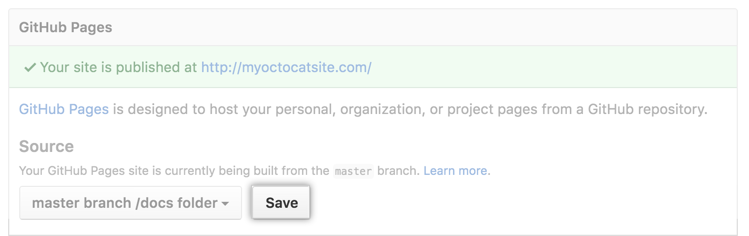
GitHub Pages will read everything to publish your site, including the
CNAME file, from the /docs folder. For example, when you edit your
custom domain through the GitHub Pages settings, the custom domain will
write to /docs/CNAME.
On GitHub, navigate to your GitHub Pages site’s repository.
Create a folder in the root of your repository on the master
branch called /docs.
Under your repository name, click Settings.
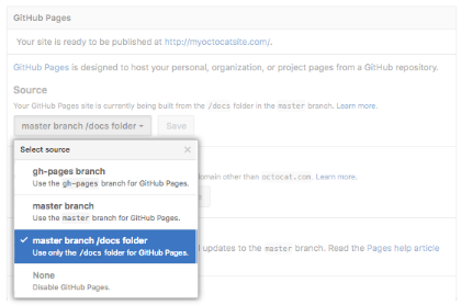
Tip: The master branch /docs folder source setting will not appear as an option if the
/docsfolder doesn’t exist on themasterbranch.
There are many many great resources on the web but linking them to a website can be hard, nont to mention boring task. Here are my notes to try and reduce the instatbility of external web links within webpages and other online content.
I am still not sure how this works exactly but here are some resources for this content.
[General tools](https://davan690.github.io/general-statistics.md)
# or
[General tools](./general-statistics.md)
Direct and indirect links??!
<div class="list-filters">
  <a href="/general-statistics" class="list-filter">Statistics</a>
  <a href="/ecological-statistics" class="list-filter">Ecology</a>
  <a href="/invasive-species-research" class="list-filter">PhD</a>
  <a href="https://www.ssnhub.com/beech-publication-wr" class="list-filter">Draft manuscript v1</a>
</div>
ReScienceC is a open source journal hosted and curated entirely on github. This journal has been active for over three years and is a interesting concept were computational reproducibility is reached and documented in a totally transparent and reproducible manner.

I have been looking into this for some time with the hope that some of New Zealands amazing
All this has been done on github commits and actions that allow for some of the editor tasks and curation to be done automatically.
Typora text editorThere are many different markdown editors to pick from but generally they range from raw txt to a “what you see is what you get” type of editor. One option for this type of editor I like is called typora.
Quick NOTE: The configuration of image file locations can be hard to get configured correctly if, in my case you don’t have a good grip of the relationship between relative and absolute paths when configuring image paths.
There was lots of press focus at the time (e.g. How NZ might make PFNZ happen;Enviroment guide; NZ geographic PFNZ plan) and academic interest too (extended info coming but most of the journal articles reference Russell et. al 2015 paper here)
 Media release in 2016 announcing New Zealands Predator Free 2050 “apollo” shot.
Although I am unsure if this is even a good idea I do know from parts of my PhD research that it will be essential that New Zealands previous research, knowledge and data will be pivotal to achieving such a goal. This research has been produced in a reproducible workflow for national-scale predator control programs.
With the continued development of my PhD work I hope to be able to connect community groups with the statistical models needed to gain the timely ecological knowledge needed to response to pest control at a national scale. I believe that this will be vital for a on-going national monitoring needed for a PFNZ by 2050.
It is possible to host a R package on github and many authors have done this. There are a collection of functions that can access packages on github by using
install.library("devtools")
library(devtools)
install.github("package_here")
library(package_here)
Here is a great package from github to look at the leading github packages:
The .bib file and the .bak file can be moved around, but the directory to the file links have to be defined accordingly. In the menu File -> Database properties, set the General file directory using a relative path, such as ./MyFiles (or .\MyFiles depending of your operating system). Afterward, you should be able to move your database and your files around.
More details here: https://help.jabref.org/en/DatabaseProperties from comment https://discourse.jabref.org/t/linked-files-cant-be-opened-after-moving-the-bak-file/211
Generating web content from different visual content types and sizes has been a challenging aspect of working with RMarkdown and document generation. I found myself saying too many times recently that I hate working with images! Image size, projection dimensions, and printing dimensions all seem to change differently at different times when working with these different image types. To break this down I have divided the different aspects and rules under each of the different content types available in RStudio using packages like rmarkdown and bookdown vs websites using jekyll.
The file location of the images matters. For different website generators and other document generators (parsers) the location of the associated files is different meaning that if images can not be found the locations defined the rendered object will no longer have an image even though you know where it is. The jekyll template
On top of this the code for accessing images and other content varies between programing languages. This means that if you do not want to use the setup I have describing here much of the content could be much more confusing than nessaracry. The tools I am using are:
Currently I am working in a dynamic HTML5 template and rendering different aspects of the original template into RMarkdown workflow for html_documents. As I have little background in such matters before now I have tried to work with existing packages and framework I manage to find in the open source community. I find it very challenging to frame up images for different blog posts, images and presentations without the following cheat guides and “work arounds”.
I thought hard and long about generating logos and other image content in R using packages like ImageMagic and others. Indeed I have opted for using a simple online editor to layout images and setting up content sizing etc for printing. For business cards and other image content it works well enough…
ImageMagic is accessed through a package called imageMagic. Working
[coming]
Over the past few months I have developed a a concept of intergrating html templates with RMarkdown to generate custom landing pages. I have used a collection of open source HTML5 templates and modified the code to include aspects of RMarkdown using $ <...> $ and custom YAML headeres associated with each of the new aspects. I have generated a template here for a dynamic CV and in the future I will extend this for other projects.
](/assets/img/method-graf.jpg)
coming soon….
Mendeley is ….. [descriptions coming soon…..]
I have now, after what seems like a lifetime, found a nice conceptial way of capturing pdf files and other resources when searching for literature. The software and tools I use are open-source and reproducible. This also means that the cost is overall very low and many of the aspects of science achievable without large cororation software such as windows, mac and other lisenced software.
[Manual coming soon….]
Tools, software, hardware, its a lot to take in but dont try and separate them anymore (cite cloud status of the world).
Organisation is key….
## Local vs remote
These are the bits that help me once I got my head around the underlying concepts:
Windows and mac so far. The linux learning curve is coming for me soon I think but I have not worked extensively in lunix yet.
These are the extensions or almost shorthand names for the applications and uses we are applying using the software. In an opensource enviroment there are alot of tools but only a few decent Software frameworks to achieve these tasks in the optonial manner (for the computer or the human as it turns out). I just think of these as the actual programs or files you have to add to your local/personal operating system to make the code or program you want to work (before packages for specific projects are added).
R is a programming language that is especially powerful for data exploration, visualization, and statistical analysis. To interact with R, we use RStudio.
| Windows | Mac OS X | Linux |
|---|---|---|
| Install R by downloading and running this .exe file from CRAN. Please also install the RStudio IDE. | Install R by downloading and running this .pkg file from CRAN. Please also install the RStudio IDE. | You can download the binary files for your distribution from CRAN. Please also install the RStudio IDE |
I have now, after what seems like a lifetime, found a nice conceptial way of working with the scientific workflow. The software and tools I use are open-source and reproducible. This comes at some costs, the main one that comes to mind is a general aspect of humanity that we can never actually get away from….if your spelling isn’t right or you math doesn’t match the current proof then its you not us….
This works for 99% of projects. The real challenge is knowning when 1% of the projects are coming up to support. Use these tools and you will work out how.
[Manual coming soon….]
Tools, software, hardware, its a lot to take in but dont try and separate them anymore (cite cloud status of the world).
These are the extensions or almost shorthand names for the applications and uses we are applying using the software. In an opensource enviroment there are alot of tools but only a few decent Software frameworks to achieve these tasks in the optonial manner (for the computer or the human as it turns out).
I just think of these as the actual programs or files you have to add to your local/personal operating system to make the code or program you want to work (before packages for specific projects are added)
Windows and mac so far. The linux learning curve is coming for me soon I think
Learning new tools (how to learn how to do things in R)
These are the bits that help me once I got my head around the underlying concepts:
## Local vs remote
This blog was build off many other researchers work but these are the ones that have come out of the woodwork as great resources for my applications:
| University of Cincinnati | |
|---|---|
| Nov 27, 2018 | Instructor: Alex Filazzola |
| 11:30 am - 1:30 pm | Co-instructors: TBD |
Statistical software that are also programming languages, such as R, are excellent tools for conducting analyses of biological data. However, many users are not taking full advantage of their capabilities. This workshop is an introduction to some of the resources that are available to R users that have been developed and implemented in the larger programming community. No prior knowledge of R will be necessary, but this workshop will not be an introduction to R basics. Instead, we will focus on using R Studio and Github to easily sync your data and analyses online. Within this workshop we will explore how to maximize reproducibility, collaborate internationally on statistical analyses, present data summaries, data management, and the promotion of open science
Who: The course is aimed at R beginners and novice to intermediate analysts. You do not need to have previous knowledge of R.
Where: University of Cincinnati: 2600 Clifton Ave, Cincinnati. 713 Rieveschl hall Map
Requirements: Participants should bring a laptop with a Mac, Linux, or Windows operating system (not a tablet, Chromebook, etc.) with administrative privileges. If you want to work along during tutorial, you must have both Git & R studio installed on your own computer (See below for instructions). However, you are still welcome to attend because all examples will be presented via a projector in the classroom.
Contact: Please contact alex.filazzola@outlook.com for more information.
LiveNotepad
| Time | Goal |
|---|---|
| 11:30 am | Meet & greet. Test software |
| 11:40 am | Github Introduction |
| 12:20 pm | Github and R Studio |
| 1:00 pm | Creating Reports with R Studio |
| 1:15 pm | Publish Reports and websites |
Please install Git before installing R Studio. This allows seamless integration between the two programs because R Studio looks for Git on your computer, but Git does not look for R Studio. In the past, installation in the opposite order has been known to create issues. If you already installed R Studio and Git, but do not see the Git Tab in R Studio then you can follow this support page to troubleshoot.
Git is a version control system that lets you track who made changes to what when and has options for easily updating a shared or public version of your code on github.com. You will need a supported web browser (current versions of Chrome, Firefox or Safari, or Internet Explorer version 9 or above).
You will need an account at github.com for parts of the Git lesson. Basic GitHub accounts are free and premium accounts are free to students. We encourage you to create a GitHub account if you don’t have one already. Please consider what personal information you’d like to reveal. For example, you may want to review these instructions for keeping your email address private provided at GitHub.
Information on how to install Git for each OS is provided by Software Carpentry and can be found here
R is a programming language that is especially powerful for data exploration, visualization, and statistical analysis. To interact with R, we use RStudio.
| Windows | Mac OS X | Linux |
|---|---|---|
| Install R by downloading and running this .exe file from CRAN. Please also install the RStudio IDE. | Install R by downloading and running this .pkg file from CRAN. Please also install the RStudio IDE. | You can download the binary files for your distribution from CRAN. Please also install the RStudio IDE |
If you enjoyed this workshop and were interested in learning more, I also run a workshop on R-basics and Introduction to Generalized Linear Modelling (GLM) found here. I also have a short introduction on using Functions in R.
You can find similar style workshops, usually that are longer and go into more detail, with Software Carpentry. They have teachers available globally and cover all forms of programming beyond R.
Dean again has made my life a lot easier than I expected. Addins are an interesting little addition to the additonal coding avaliable under the RStudio platform.
#include html readme here...
#devtools::install_github("rstudio/addinexamples", type = "source")
A good basic readme document and webpage can be found at https://rstudio.github.io/rstudioaddins/#overview.
I have been thinking about this as a good way to manage the risk associated with using other peoples addins without understanding the functions they are implmenting in your local enviroment…. a blog extension will be coming soon…..
iframes#using knitr
gists[coming]
#list packages
Prose.io is a web app that allows the user to access there github content. In other words prose is “a content editor for GitHub”.
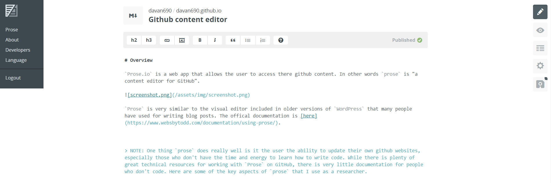
Prose is very similar to the visual editor included in older versions of WordPress that many people have used for writing blog posts. The offical documentation is here.
NOTE: One thing
prosedoes really well is it the user the ability to update their own github websites, especially those who don’t have the time and energy to learn how to write code. While there is plenty of great technical resources for working withProseon GitHub, there is very little documentation for people who don’t code. Here are some of the key aspects ofprosethat I use as a researcher.
Prose allows simple draft post creation for github (and jekyll) through a web app/interface for simple markdown. Markdown is very easy to learn as it is ment to be read as plain text as well as rendered as a document like word or html. See my early post for some basics
I really just use it to enter the text and ideas for blogs. It makes it easier to sit in a cafe and write an idea down that then can be included as a blog post or documentation for a project I am working on. I like using it at the moment because I have been able to test the effectiveness of my markdown code to render the posts and information I use regularly in R. A couple of key points that make prose good:
Makes automatic commit lines when you save
Shortcut for saving in windows ctrl s works as a automatic commit making it easy to update draft after you have made comments
Easy for short passages of text == good for a blog
Uses markdown which results in much easier inclusion in other markdown flavours such as RMarkdown
Maybe in the future this will be a good tool to get simple ideas from the notepad to the publication level quicker?
Here is a simple step-by-step guide to editting blogs using github and prose online.
Open web browser and navigate to: https://prose.io/
Authenticate your github account associated with the blog site you want to work on.
Navigate to the repository where your blog is kept.
Generate a new post. NOTE: this will be saved in the _drafts folder until published.
This is a nice quick way to generate a new blog template and file.
./_posts/ folder of your blogs repository.There are a collection of functions and packages I have been using recently to access the citizen science data repository of Koala observations (the amazing ALA).
There are many tools that access and use the data associated with the ALA. To find an updated list of them in all their glory see the ALA website website here.
In particular I have been using the spatial portal to visualise the data and then think about the best way to capture this information directly from the API (through a package like galah is great). There are some challenges with this workflow but I have managed to make it work for the first few pieces of work now and I hope it will get quicker.
I have found that the galah package is very easy to capture and investigate particular sections of the database. Here are a few snippets of code that I have been using:
[rcode here]
There are several ways that it is possible to generate static html content that includes aspects of different social media posts and pages. Here are a few quick notes about how I work with these file formats.
iframeThe iframe function can be used for many of these aspects as so…..
[insert table of options]
Google has a huge wealth of location data. It is possible to access and use this data in a range of ways. Here is some information on using iframe in a markdown or rmarkdown document. Here is the beginning of what I hope will be a collection of R scripts and notes on how to deal with google location data in R. Mostly because I have found this hard and I hope by writing a bunch of blog posts about it I will become more accustom to working with this sort of data.
iframeiframe is one of the easiest way to embed an interactive web application inside a html webpage. In short, put maps in your documents from other applications online such as the my-maps map I have created below:
<iframe src="<YOUR_LINK HERE>" width="600" height="450" style="border:0;" allowfullscreen="" loading="lazy"></iframe>
I have been trying to use and write functions instead of loops in R and this is what I have for a customised iframe function for jekyll posts below. I ahve tried to make it as simple as possible as a function example too.
#parameters
urladd <- "https://www.google.com/maps/embed?pb=!1m18!1m12!1m3!1d102728.53602889985!2d149.96889269268158!3d-36.42693204654719!2m3!1f0!2f0!3f0!3m2!1i1024!2i768!4f13.1!3m3!1m2!1s0x6b3e721c18d3ea21%3A0x40609b4904406a0!2sBermagui%20NSW%202546!5e0!3m2!1sen!2sau!4v1625880170565!5m2!1sen!2sau"

##function
#iframeFUNC <-
#function(urladd){
#how to include html snippet in function call RMD?
#<iframe src=urladd width="600" height="450" style="border:0;" allowfullscreen="" loading="lazy"></iframe>
#}
iframeThe same iframe code can be used for a shiny app hosted on the rstudio shiny server (5 free apps as of June 2021). There is also a package to make uploading and publishing your shiny app much easier here These resources are great tools for accessing and communicating early development of RShiny apps over the web. Additional, if you feel bold golem is great for shiny development as a package here.
<iframe
	src=<"YOUR-SHINY-APP">
	width=<"MEASUREMENT">
    height=<"MEASUREMENT">
    style="border:0;"
    allowfullscreen=""
    loading="lazy">
 </iframe> # finish code
And then it can look something like this:
</div>
The trove database is a amazing resource that is configured using a simple API. There is a tool called QueryPic that can be used from within an online jupyter notebook that makes working with the overall data from TROVE much easier.
The credit I can find so far goes to WraggeLabs: Tim Sherratt and GLAM workbench. Let me know if I have missed key contributors please. :)
include info here from page??
In a perfect world I could be able to write all my code as vectorised functions. This is a helpful tutorial for the overall concept.
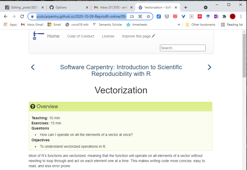
During the first 6 months of 2021 I was lucky enough to help out with a course called “Big Questions in Biology”. I have broken up a lot of the resources I used in the class and added them as smaller blog posts to this site for now. Any feedback is great. :).
covid19 cases/trendsThe overall world data has been curated by (“Our World in Data”](https://ourworldindata.org/). The tabs on the bottom of the window below navigate the original site here: https://ourworldindata.org/grapher/covid-confirmed-cases-since-100th-case?country=NZL+KOR+AU
I found this great shiny app that I have managed to reproduce on my shiny server. The next step is to recreate it with some new or different data. Link here.
[iframe here]
I have been slowly working on the development of a similar approach to some of the data I work with. I have added this information in combination with other open repositories and resources.
Here are some other posts associated with this work.
| <div>
</div> | This repository is a combination of several shiny tutorials and and the framework from the US parks shiny app here … |
| Personal draft resources | Hosted on github |
Please excuse any ‘404’ errors as I am learning and working as I go. Using version control and git means that I am able to use other coders templates and test things out before committing.
</html>
GIS is an area of R coding I have kept away from hoping that I would work it out at a later date. Sadly, it has got to the point where I want to be able to build more complex maps in shiny applications towards the end of my PhD and need to create a base of code to go from. Luckily, the text book “Spatial Analysis in R” has just come out in its second edition and is available in as a bookdown repository including the full text here.
This page is a outline of the current resources I am working on and using for my publication and website maps. I have begun by using my normal reproducible workflow and file structure. The full set of resources is currently on a private repository where the resources can be found in the following layout:
a stack-overflow feed is easier to find the answers in. A good start to begin to build RMarkdown documents quickly.I hate to think currently but there are many options around this using a range of workflows. The final copy will render to ‘PDF’ and each chapter draft will be edited etc in docx files. This is all possible however rendering the entire thesis as one in word is likely to have issues. IF this will be a problem I will need to sort this as soon as possible.
This is a demo post to show you how to write blog posts for jekyll websites using markdown. I strongly encourage you to take 5 minutes to learn how to write in markdown - it’ll teach you how to transform regular text into bold/italics/headings/tables/etc. For a more detailed guide see https://www.markdownguide.org/.
Markdown is a plain text language meaning that
Here is some bold text
Here’s a useless table:
| Number | Next number | Previous number |
|---|---|---|
| Five | Six | Four |
| Ten | Eleven | Nine |
| Seven | Eight | Six |
| Two | Three | One |
How about a yummy crepe?

It can also be centered!
Here’s a code chunk:
var foo = function(x) {
  return(x + 5);
}
foo(3)
And here is the same code with syntax highlighting:
var foo = function(x) {
  return(x + 5);
}
foo(3)
And here is the same code yet again but with line numbers:
1
2
3
4
var foo = function(x) {
  return(x + 5);
}
foo(3)
You can add notification, warning and error boxes like this:
Note: This is a notification box.
Warning: This is a warning box.
Error: This is an error box.
Under what circumstances should we step off a path? When is it essential that we finish what we start? If I bought a bag of peanuts and had an allergic reaction, no one would fault me if I threw it out. If I ended a relationship with a woman who hit me, no one would say that I had a commitment problem. But if I walk away from a seemingly secure route because my soul has other ideas, I am a flake?
The truth is that no one else can definitively know the path we are here to walk. It’s tempting to listen—many of us long for the omnipotent other—but unless they are genuine psychic intuitives, they can’t know. All others can know is their own truth, and if they’ve actually done the work to excavate it, they will have the good sense to know that they cannot genuinely know anyone else’s. Only soul knows the path it is here to walk. Since you are the only one living in your temple, only you can know its scriptures and interpretive structure.
At the heart of the struggle are two very different ideas of success—survival-driven and soul-driven. For survivalists, success is security, pragmatism, power over others. Success is the absence of material suffering, the nourishing of the soul be damned. It is an odd and ironic thing that most of the material power in our world often resides in the hands of younger souls. Still working in the egoic and material realms, they love the sensations of power and focus most of their energy on accumulation. Older souls tend not to be as materially driven. They have already played the worldly game in previous lives and they search for more subtle shades of meaning in this one—authentication rather than accumulation. They are often ignored by the culture at large, although they really are the truest warriors.
A soulful notion of success rests on the actualization of our innate image. Success is simply the completion of a soul step, however unsightly it may be. We have finished what we started when the lesson is learned. What a fear-based culture calls a wonderful opportunity may be fruitless and misguided for the soul. Staying in a passionless relationship may satisfy our need for comfort, but it may stifle the soul. Becoming a famous lawyer is only worthwhile if the soul demands it. It is an essential failure if you are called to be a monastic this time around. If you need to explore and abandon ten careers in order to stretch your soul toward its innate image, then so be it. Flake it till you make it.
| Fork | Branch | Notes |
|---|---|---|
 |
master | This is the branch I am currently working on |
 |
master | |
 |
master |
You can host your book on GitHub for free via GitHub Pages (https://pages.github.com). GitHub supports Jekyll (http://jekyllrb.com), a static website builder, to build a website from Markdown files. That may be the more common use case of GitHub Pages, but GitHub also supports arbitrary static HTML files, so you can just host the HTML output files of your book on GitHub. The key is to create a hidden file .nojekyll that tells GitHub that your website is not to be built via Jekyll, since the bookdown HTML output is already a standalone website.
# assume you have initialized the git repository,
# and are under the directory of the book repository now

# create a hidden file .nojekyll
touch .nojekyll

# add to git here because will not show up in RStudio
git add .nojekyll
If you are on Windows, you may not have the touch command, and you can create the file in R using file.create('.nojekyll').
One approach is to publish your book as a GitHub Pages site from a /docs folder on your masterbranch as described in GitHub Help. First, set the output directory of your book to be /docs by
adding the line output_dir: "docs"
to the configuration file _bookdown.yml.
Then, after pushing your changes to GitHub,
go to your repository’s settings and
under “GitHub Pages” tab
change the “Source”
to be “master branch /docs folder”.
In this case, the .nojekyll file has to be in the /docs folder.
#create.file("docs/", ".nojekyll")
The interesting thing about this post is that this is not exactly what I am hoping for as an end product. only possible because of these tools (leaflet; wiki on the matter and shiny info).
To begin with check this is working in your local RStudio enviroment
GEOS, Proj.4, and UDUNITS libraries installed for this to work on Mac and Linux. More information on that at https://github.com/r-spatial/sf.devtools::install_github("robinlovelace/geocompr")
library(spData)library(dplyr)library(sf)
world %>% plot()
And some blogging on the matter here.
Leaflet supports basemaps using map tiles, popularized by Google Maps and now used by nearly all interactive web maps.
The easiest way to add tiles is by calling addTiles() with no arguments; by default, OpenStreetMap tiles are used.
```{r fig.height=2.5} m <- leaflet() %>% setView(lng = -71.0589, lat = 42.3601, zoom = 12) m %>% addTiles()
### Third-Party Tiles

Alternatively, many popular free third-party basemaps can be added using the `addProviderTiles()` function, which is implemented using the [leaflet-providers plugin](https://github.com/leaflet-extras/leaflet-providers). See [here](http://leaflet-extras.github.io/leaflet-providers/preview/index.html) for the complete set.

As a convenience, leaflet also provides a named list of all the third-party tile providers that are supported by the plugin. This enables you to use auto-completion feature of your favorite R IDE (like RStudio) and not have to remember or look up supported tile providers; just type `providers$` and choose from one of the options. You can also use `names(providers)` to view all of the options.

```{r fig.height=1.25}
m %>% addProviderTiles(providers$Stamen.Toner)
m %>% addProviderTiles(providers$CartoDB.Positron)
m %>% addProviderTiles(providers$Esri.NatGeoWorldMap)
Note that some tile set providers require you to register; see the project page for more information. You can pass access tokens/keys, and other options, to the tile provider by populating the options argument with the providerTileOptions() function.
If you happen to have a custom map tile URL template to use, you can provide it as an argument to addTiles().
You can use addWMSTiles() to add WMS (Web Map Service) tiles. The map below shows the Base Reflectivity (a measure of the intensity of precipitation occurring) using the WMS from the Iowa Environmental Mesonet :
```{r fig.height=2.5} leaflet() %>% addTiles() %>% setView(-93.65, 42.0285, zoom = 4) %>% addWMSTiles( “http://mesonet.agron.iastate.edu/cgi-bin/wms/nexrad/n0r.cgi”, layers = “nexrad-n0r-900913”, options = WMSTileOptions(format = “image/png”, transparent = TRUE), attribution = “Weather data © 2012 IEM Nexrad” )
### Combining Tile Layers

You aren't restricted to using a single basemap on a map; you can stack them by adding multiple tile layers. This generally only makes sense if the front tiles consist of semi transparent tiles, or have an adjusted opacity via the `options` argument.

```{r fig.height=1.75}
m %>% addProviderTiles(providers$MtbMap) %>%
  addProviderTiles(providers$Stamen.TonerLines,
    options = providerTileOptions(opacity = 0.35)) %>%
  addProviderTiles(providers$Stamen.TonerLabels)
Making choropleths with leaflet is easy. In this example, we’ll duplicate the step-by-step choropleth tutorial from the Leaflet.js website.
The final result will look like this (scroll to the end to see the completed code):
```{r fig.height = 4.75, echo = FALSE}
states <- geojsonio::geojson_read(“./json/us-states.geojson”, what = “sp”)
bins <- c(0, 10, 20, 50, 100, 200, 500, 1000, Inf)
pal <- colorBin(“YlOrRd”, domain = states$density, bins = bins)
labels <- sprintf(
“%s
%g people / mi2”,
states$name, states$density
) %>% lapply(htmltools::HTML)
leaflet(states) %>%
setView(-96, 37.8, 4) %>%
addProviderTiles(“MapBox”, options = providerTileOptions(
id = “mapbox.light”,
accessToken = Sys.getenv(‘MAPBOX_ACCESS_TOKEN’))) %>%
addPolygons(
fillColor = ~pal(density),
weight = 2,
opacity = 1,
color = “white”,
dashArray = “3”,
fillOpacity = 0.7,
highlight = highlightOptions(
weight = 5,
color = “#666”,
dashArray = “”,
fillOpacity = 0.7,
bringToFront = TRUE),
label = labels,
labelOptions = labelOptions(
style = list(“font-weight” = “normal”, padding = “3px 8px”),
textsize = “15px”,
direction = “auto”)) %>%
addLegend(pal = pal, values = ~density, opacity = 0.7, title = NULL,
position = “bottomright”)
### Data source

We'll start by loading the data from JSON. While the Leaflet.js example loads the JSON directly into JavaScript, with the Leaflet R package we instead want to load the data into R.

In this case, we'll use the `geojsonio` package to load the data into `sp` objects, which will let us easily manipulate the geographic features, and their properties, in R.

```{r}
states <- geojsonio::geojson_read("json/us-states.geojson", what = "sp")
class(states)
names(states)
As you can see, we now have a SpatialPolygonsDataFrame with name (state name) and density (population density in people/mi2) columns from the GeoJSON.
Next, let’s make a basic map with just the outline of the states. For our basemap, we’ll use the same "mapbox.light" MapBox style that the example does; if you don’t have a MapBox account, you can just use addTiles() in place of the addProviderTiles call, or choose a free provider.
m <- leaflet(states) %>%
  setView(-96, 37.8, 4) %>%
  addProviderTiles("MapBox", options = providerTileOptions(
    id = "mapbox.light",
    accessToken = Sys.getenv('MAPBOX_ACCESS_TOKEN')))
We’ve saved the basic basemap as a separate variable m so we can easily iterate on the addPolygons call as we work through the rest of the tutorial.
To add uniform polygons with default styling, just call addPolygons with no additional arguments.
m %>% addPolygons()
Now, let’s color the states according to their population density. You have various options for mapping data to colors; for this example we’ll match the Leaflet.js tutorial by mapping a specific set of bins into RColorBrewer colors.
First, we’ll define the bins. This is a numeric vector that defines the boundaries between intervals ((0,10], (10,20], and so on).
Then, we’ll call colorBin to generate a palette function that maps the RColorBrewer "YlOrRd" colors to our bins.
Finally, we’ll modify addPolygons to use the palette function and the density values to generate a vector of colors for fillColor, and also add some other static style properties.
bins <- c(0, 10, 20, 50, 100, 200, 500, 1000, Inf)
pal <- colorBin("YlOrRd", domain = states$density, bins = bins)
m %>% addPolygons(
  fillColor = ~pal(density),
  weight = 2,
  opacity = 1,
  color = "white",
  dashArray = "3",
  fillOpacity = 0.7)
The next thing we’ll want is to make the polygons highlight as the mouse passes over them. The addPolygon function has a highlight argument that makes this simple.
m %>% addPolygons(
  fillColor = ~pal(density),
  weight = 2,
  opacity = 1,
  color = "white",
  dashArray = "3",
  fillOpacity = 0.7,
  highlight = highlightOptions(
    weight = 5,
    color = "#666",
    dashArray = "",
    fillOpacity = 0.7,
    bringToFront = TRUE))
(The Leaflet.js tutorial also adds an event handler that zooms into a state when it’s clicked. This isn’t currently possible with the Leaflet R package, except with either custom JavaScript or using Shiny, both of which are outside the scope of this example.)
Now let’s expose the state names and values to the user.
The Leaflet.js tutorial shows the hovered-over state’s information in a custom control. Again, that’s possible by adding custom JavaScript or using Shiny, but for this example we’ll use the built-in labels feature instead.
We’ll generate the labels by handcrafting some HTML, and passing it to lapply(htmltools::HTML) so that Leaflet knows to treat each label as HTML instead of as plain text. We’ll also set some label options to improve the style of the label element itself.
labels <- sprintf(
  "<strong>%s</strong><br/>%g people / mi<sup>2</sup>",
  states$name, states$density
) %>% lapply(htmltools::HTML)
m <- m %>% addPolygons(
  fillColor = ~pal(density),
  weight = 2,
  opacity = 1,
  color = "white",
  dashArray = "3",
  fillOpacity = 0.7,
  highlight = highlightOptions(
    weight = 5,
    color = "#666",
    dashArray = "",
    fillOpacity = 0.7,
    bringToFront = TRUE),
  label = labels,
  labelOptions = labelOptions(
    style = list("font-weight" = "normal", padding = "3px 8px"),
    textsize = "15px",
    direction = "auto"))
m
This is the final version of our polygon layer, so let’s save the result back to the m variable.
As our final step, let’s add a legend. Because we chose to color our map using colorBin, the addLegend function makes it particularly easy to add a legend with the correct colors and intervals.
m %>% addLegend(pal = pal, values = ~density, opacity = 0.7, title = NULL,
  position = "bottomright")
```{r results = ‘hide’}
states <- geojsonio::geojson_read(“json/us-states.geojson”, what = “sp”)
bins <- c(0, 10, 20, 50, 100, 200, 500, 1000, Inf)
pal <- colorBin(“YlOrRd”, domain = states$density, bins = bins)
labels <- sprintf(
“%s
%g people / mi2”,
states$name, states$density
) %>% lapply(htmltools::HTML)
leaflet(states) %>%
setView(-96, 37.8, 4) %>%
addProviderTiles(“MapBox”, options = providerTileOptions(
id = “mapbox.light”,
accessToken = Sys.getenv(‘MAPBOX_ACCESS_TOKEN’))) %>%
addPolygons(
fillColor = ~pal(density),
weight = 2,
opacity = 1,
color = “white”,
dashArray = “3”,
fillOpacity = 0.7,
highlight = highlightOptions(
weight = 5,
color = “#666”,
dashArray = “”,
fillOpacity = 0.7,
bringToFront = TRUE),
label = labels,
labelOptions = labelOptions(
style = list(“font-weight” = “normal”, padding = “3px 8px”),
textsize = “15px”,
direction = “auto”)) %>%
addLegend(pal = pal, values = ~density, opacity = 0.7, title = NULL,
position = “bottomright”)
```
https://www.canva.com/design/DAE47TyDc_s/LkWFUEh_Wmtod7HqSh58ww/view?utm_content=DAE47TyDc_s&utm_campaign=designshare&utm_medium=link&utm_source=shareyourdesignpanel
As I am finishing up my PhD and working out how to build a career in academia I have ran out of money and resources in the long drawn-out finishing line.
I have also been noticing that I am losing connections (both for work and by not having a business card to direct people to the website when suites them. We have little support in these sorts of areas as graduate students and even less funding . As a graduate student I got the generic card when I asked and since our institute has been incorporated into the universities science department I don’t even dear ask.
So instead I have built this website but now I still don’t have cash for business cards (really just networking tools here) yet even though I have the resource.
This is my solution to business cards with an quirky edge or, as some would say, a student budget.

I have put together a very rough logo in the center and added my contact details to a single label template. I found this one below with a very quick google search so I’m sure there are better solutions with some more time however this one:


I then printed the image which gave me a pdf to download or print. Which leads to a pdf of 36 labels ready to print for 50c in colour printing.

I am not sure if I can just stick these onto politicians wasted junk mail or not?
<–image of cards being used as card for stickers–>
The labels are expensive but it still works out to be less than …. cents a card and since we are recycling and saving $$.
I figure its a win or at least a stop-gap until I find another funding source.
As with all github projects there always seems to be someone else who has managed to explain and write a blog about what you need, just when you need it… I wish :)
This is an collection of resources I have used to make this happen. I think this is a massive leap for reproducible workflow and in particular, science commumication but I will build on this thoughout the website.
I found this blog explaining how Jacob Fiksel steps through the process very helpful.
These are my take home points and things I found hard.
Need all the basics to begin with (GIThub, Jekyll, R, RStudio).
Key run code
??bundle gem install jekyll??

bundle exec jekyll build

bundle exec jekyll serve --watch
> servr::jekyll()

Serving the directory C:\GIT\davan690.github.io at http://127.0.0.1:5652
servr::daemon_stop(3)
Warning message:
In system2("jekyll", "build"):
'"jekyll"' not found NULL
I found I needed to install ruby gems for jekyll using the following code snippits:
??bundle gem install jekyll??
The compareGroups package (Subirana, Sanz, and Vila 2014) allows users to create tables displaying results of univariate analyses, stratified or not by categorical variable groupings.
Tables can easily be exported to CSV, LaTeX, HTML, PDF, Word or Excel, or inserted in R-markdown files to generate reports automatically.
This package can be used from the R prompt or from a user-friendly graphical user interface for non-R familiarized users.
The compareGroups package is available on CRAN repository. To load the package using the R prompt, enter:
library(compareGroups)I have developed this slightly in my notes as function used for quick descriptive statistics using R and a GUI. For now these notes are on this page. At some stage I plan to move these to there own repository.
To access the GUI there are several additional packages that are needed so that a interactive window can be opened by RStudio. However, these packages will already be running if you have other similar functions within your library already.
# compareGroups::cGroupsGUI(mtcars)There is a very good vignette for this package here. This document provides an overview of the usage of the compareGroups package with a real examples, both using the R syntax and the graphical user interface. It is structure as follows: Overall, there is a introduction of the package (section 2) and the data used as example (section 3), Instructions to perform descriptive tables and exploration plots using R syntax are explained (section 4), and Usage of graphical user interface based on tcl-tk (section 5) and based on Shiny (section 6) are shown.
A KMZ file is just a zipped KML file, possibly with associated embedded images, icons, etc. So any program that supports KMZ files internally unzips them to access their KML files. That may be a reason why many open source programs do not bother supporting KMZ once KML support is implemented: you just need to use an additional unzipping library of your choice, to convert the KMZ to KML. The linked posts give some JavaScript-based solutions for unzipping.
I like the idea of sticking with this process so that “google” will manage the security of the data instead of any open-source tools with security issues.
We need to convert the my-maps data from a zipped kml file that is stored as the kmz file downloaded from mymaps data.
kmz conversionFollow these steps:
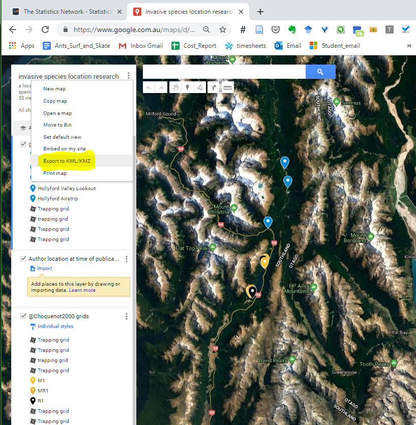
.zip to .kml filekmz##librares needed
library(rgdal)
library(tidyverse)
library(ggplot2)
```{r kmzKml} nc <- st_read(system.file(“shape/nc.shp”, package=”sf”), quiet = TRUE)
nc <- nc[1:2,]
nc_sp <- as(nc, “Spatial”)
file <- “data/Canberra-Transit.kmz/doc.kml”
?readOGR SST_start = readOGR(file)
SST_1 = readOGR(file,”SST_1”) OGR data source with driver: LIBKML Source: “Burrows_et_al_Nature_traj_ocean_NH1.kmz”, layer: “SST_1” with 7719 features It has 12 fields ```
Found in stack comments here
Somehow a few months ago I managed to add google analytics to both my blog website here and my first publication but I am unsure how I managed it.
I have now come back to this as I need to set up google analytics for a custom html website with a single landing page.
I was hesitant to get this all working due to having to get involved with google and things like google adwords. For now I only have inserted the single google analytics code for my personal site. It is not much harder to add additional tracking tags using google’s tag tracker.
I have collected a few resources to setup another page with google analytics. It is helpful to therefore have a google account setup for the project. There are limitations to the use of google however it can be helpful to upgrade if projects get bigger or more security savvy.
A KMZ file is just a zipped KML file, possibly with associated embedded images, icons, etc. So any program that supports KMZ files internally unzips them to access their KML files. That may be a reason why many open source programs do not bother supporting KMZ once KML support is implemented: you just need to use an additional unzipping library of your choice, to convert the KMZ to KML. The linked posts give some JavaScript-based solutions for unzipping.
These resources are very basic but they may be helpful for me later.
Found in stack comments here
KMZ files are just… (21 May 2019)
Example states for shiny-salesman app….
# From http://leafletjs.com/examples/choropleth/us-states.js
# Data Referenced from https://github.com/rstudio/leaflet/tree/master/docs/json/

states <- geojsonio::geojson_read("./json/us-states.geojson", what = "sp")
bins <- c(0, 10, 20, 50, 100, 200, 500, 1000, Inf)
pal <- colorBin("YlOrRd", domain = states$density, bins = bins)
labels <- sprintf(
  "<strong>%s</strong><br/>%g people / mi<sup>2</sup>",
  states$name, states$density
) %>% lapply(htmltools::HTML)
leaflet(states) %>%
  setView(-96, 37.8, 4) %>%
  addProviderTiles("MapBox", options = providerTileOptions(
    id = "mapbox.light",
    accessToken = Sys.getenv('MAPBOX_ACCESS_TOKEN'))) %>%
  addPolygons(
    fillColor = ~pal(density),
    weight = 2,
    opacity = 1,
    color = "white",
    dashArray = "3",
    fillOpacity = 0.7,
    highlight = highlightOptions(
      weight = 5,
      color = "#666",
      dashArray = "",
      fillOpacity = 0.7,
      bringToFront = TRUE),
    label = labels,
    labelOptions = labelOptions(
      style = list("font-weight" = "normal", padding = "3px 8px"),
      textsize = "15px",
      direction = "auto")) %>%
  addLegend(pal = pal, values = ~density, opacity = 0.7, title = NULL,
    position = "bottomright")
This is an extension of the demo post from Dean’s website that demostrates some key markdown syntax to use in markdown blog posts for this site (and many other great tools).
There are many resources and blogs about how to use markdown. Here is a 5 minutes guide to writing in markdown - it’ll teach you how to transform regular text into bold/italics/headings/tables/etc. Here are some quick notes.
Bold text is defined by **: Here is some bold text
Headings are defined by the number of # before a line of text. For example ##### Here is a fifth level heading is needed and then the rendered document will have a fifth level heading as below.
##))and a sixth heading by ######. This is the max level for a heading by the way…
One of the greatest strengths of markdown extensions such as RMarkdown is the ability to include code chunks within normal text as below:
var foo = function(x) {
  return(x + 5);
}
foo(3)
And here is the same code with syntax highlighting:
var foo = function(x) {
  return(x + 5);
}
foo(3)
And here is the same code yet again but with line numbers:
1
2
3
4
var foo = function(x) {
  return(x + 5);
}
foo(3)
You can add notification, warning and error boxes like this:
{: .box-note} ; {: .box-warning}; {: .box-error} demos below:
Note: This is a notification box.
You can set following yaml variables: layout: post; tags: <tagg_label>
Images live in the ./assets/img/ folder following the same rules as the beautiful jekyll template. Overall jekyll uses liquid tags to and these usually found in the assets folder.
How about a yummy crepe? Here are two sections of code for working with markdown syntax (code). It can also be centered using {: .mx-auto.d-block :}
Tables can be directly written using markdown syntax or can be built in code and rendered to markdown using a package like knitr in R.
Markdown tablesMarkdown tables can be difficult to keep formatted. Here’s a demo markdown table:
| Number | Next number | Previous number |
|---|---|---|
| Five | Six | Four |
| Ten | Eleven | Nine |
| Seven | Eight | Six |
| Two | Three | One |
RMarkdown tablesAn advantage of RMarkdown is that you can build autogenerating markdown tables using a range of packages including knitr.
Although this site is just a collection of blog posts and notes about working with open science frameworks it can also be something else. I think that there are a collection of additional aspects to the same workflow and tools I am using here to produce reproducible graduate research. With the combination of comments, notes and live editting it should be possible to add and work on content in a dynamic and collaborative way using version control, R and the associated tools within these frameworks for computer software development.
To test this concept I have begin by working online as much as I can and submitting or “publishing” content that is still in draft/uncompleted form so that as I intergrate the key tools needed in the future, I can begin to add comments and extend content in a more community driven manner.
```
An easy way to find what I am on about is to use ctrl/command + F in chrome on any webpage and search….
[insert image here…]


